|
|
Analysis of
Elliptical Galaxies |
|||||
|
This
analysis is part of a sequence of logical steps that are described in Investigation. The density/radius relationship of elliptical
galaxies is not claimed to be evidence for antigravity matter. However the objective of this page is to
demonstrate that it is also not evidence against antigravity matter. Prediction According
to the AGM Theory most elliptical galaxies should be a little below the large
scale AGM Exclusion Density which should be independent of radius. This is because :-
|
|
Data Source and Calculation To test this prediction elliptical galaxy data were
acquired from Hyperleda using
the sql statement “select *
where objtype='G' and type='E'”. Galaxies were removed from the sample with
negative or no recession velocity data, or with no brightness or radius
data. This left 3408 galaxies. The following calculations were performed:-
Most of this calculation is well known and obvious but
some special considerations are described below. |
|
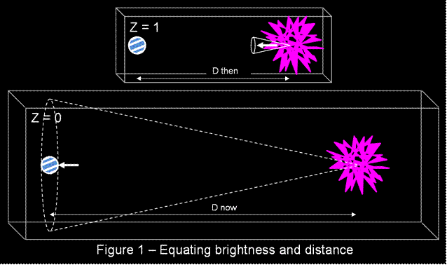
In Figure 1 a pulse of light starts from a distant
galaxy at the time of z = 1. At that
time the distance between the galaxy and the earth (D then) was half what it
is now (D now). At the time of z = 0
(the present) the light arrives at the earth and the luminance of the light
pulse is measured. It can be seen from
Figure 1 that if we are to equate absolute brightness, apparent brightness
and distance we must use D now. D now
dictates how much the pulse has spread out.
This applies for any positive value of z. Hubble’s Law has been validated using the apparent
brightness of Cepheid variables and other bightness
related techniques (source). We therefore assume that Hubble’s Law gives
an estimate of D now. |
|
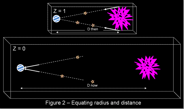
The universe expands while the light beams are
travelling. Despite this expansion
straight lines remain straight. The
light beams were moving in the direction of the Earth at the start, and
arrive at the Earth at the time of z = 0.
The angle between the two light beams is measured. It can be seen from Figure 2 that if we are to equate
angular size, actual size and distance we must use D then. This applies for any positive value of z. |
|
As a result of the argument above the absolute
brightness and therefore the mass of the galaxy is calculated using D now but
the radius of the galaxy is calculated using D then. |
|
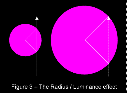
In the original
data the angular size of each galaxy is measured to the isophote
(contour of constant luminance) at which luminance is 25 mag.arcsec-2. However the length of a geometrically
similar line of sight through a spherical object increases as the radius of
the object increases as depicted in Figure 3 on the right. As a result the average (3 dimensional)
density along the line of sight that passes through the 25 mag.arcsec-2
isophote reduces as the galaxy radius
increases. To allow galaxies of
different sizes to be compared the radius calculation must take account of
this Radius / Luminance effect. |
|
Therefore we apply a correction to the radius such
that:- Corrected Radius = Radius ×
(10000 ly / Radius (ly))Fr Where Fr is
a correction parameter with a starting guess of ¼. This value corresponds with a guess that
for a 10000 ly radius galaxy the radius of the 25
mag.arcsec-2 isophote is somewhat greater than Re at a
radius where luminance is inversely proportional to the forth power of
radius. Later we investigate the
effect of adjusting the value of Fr. The figure
10000 ly is chosen arbitrarily. This means that the definition of radius is
also arbitrary, but since the original definition of radius (the 25 mag.arcsec-2 isophote) was also arbitrary this has no
real effect. We are generating a
radius value that allows galaxies of different size to be compared. This is not the radius of the AGM Boundary,
though we are assuming that the AGM Boundary is nearby in the outer
extremities of the galaxy. |
|
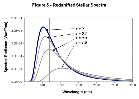
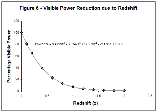
Consideration 3 – Redshifting A typical
star has approximately the radiation spectrum of a black body at a
temperature of 5523 K (source). As the light from a star is redshifted it
moves out of the visible range. In
addition each photon loses energy as its wavelength increases. Figure 5 shows several spectra from such a
black body that have been redshifted by varying amounts. The amount of energy in the visible range
between blue and red vertical lines reduces as z increases. We use this graph to explore the
relationship between visible light and redshifting. This leads to the points on the graph shown
in Figure 6. We derive a forth power
polynomial to define the trendline fitted to the
data points as shown.
This polynomial is then used to generate a Brightness
Multiplication Factor which is used in the calculation of the absolute
brightness and therefore the mass of the galaxies. If galaxy brightness is increased by the above argument
then galaxy radius must also be increased because radius is measured at a
particular isophote as described above.
The following is included in the radius calculation:- Corrected Radius = Radius calculated so far ×
(Brightness Multiplication Factor)Fr Where Fr is
the correction parameter with a starting guess of ¼ as described in
Consideration 2 above. . |
|
Results The
following graphs are produced.
|
|
Observations and Concerns The
concerns listed from 3) onwards below are not believed to be evidence against
the antigravity matter theory. They
all relate to observations over very large distances and may be clues to
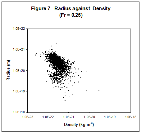
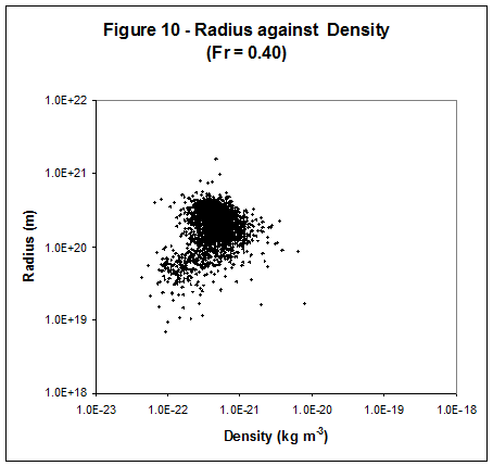
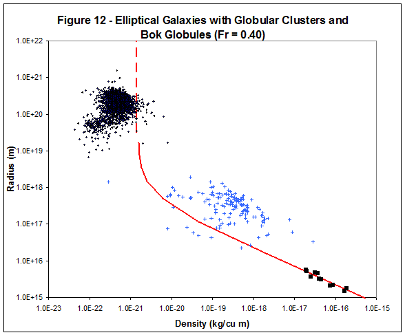
other cosmological effects. 1) Figure 7 shows that with the guessed
value of Fr = 0.25 the range of most elliptical galaxy densities is less than
one decade. Figure 10 shows that with
a higher value of Fr = 0.4 the majority of elliptical galaxies are even more
tightly grouped. Figure 12 shows them
in the context of the red Dnx line as generated in Investigation.
The Dnx line runs vertically to the right of the elliptical galaxies
because the AGM Boundary is assumed to be within the calculated radius of the
galaxy. 2) When Fr = 0.4 smaller elliptical
galaxies are less dense. It may be
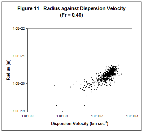
that these galaxies are actually falling apart. This would be consistent with Figure 11
which shows that below a galaxy radius of about 1 ×10²⁰
m (~10000 ly)
dispersion velocity appears to fall dramatically, suggesting that the stars
in these galaxies are less constrained by gravity. If this were the case the majority of the
stars in these galaxies are in the AGM Mixed state as described in Behaviour. 3) It is worrying that the majority of
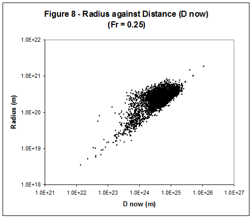
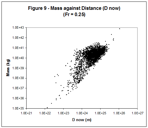
the galaxies also appear to have a limited range of radii. 4) It is also worrying that maximum
galaxy radius and maximum galaxy mass appear to increase with distance as
shown in Figures 8 and 9. For the most
distant galaxies z ~ 0.8 so we are observing these as they were when the
universe was significantly younger.
This suggests the maximum size of elliptical galaxies has been getting
smaller for a long time. 5) It is also worrying that if the
amount of antigravity matter in the universe was constant and if Gnn, Gna and
Gaa remained constant we would actually expect the AGM Exclusion Density to
be higher in the distant past. At z =
1 we would expect the AGM Exclusion Density to be 8 times higher. This does not come out of the data. |
© Copyright Tim E Simmons 2008 to
2015. Last updated 28th July 2015.
Major changes are logged in AGM
Change Log.